Model Overview

Inputs (X)

For a player, a stats input is generated each month, as well as one upon player signing. When a player plays at multiple levels in a given year, the stats are combined, with the level being the weighted average of the levels for the month. All stats are normalized to the league at which the player is at, so rather than having a player's AVG, it instead has their AVG as a multiple of the average AVG at that league for that period.

The following stats are used to create the inputs

Both

• Age at signing
• Draft Pick
• Draft Signing Rank
• Age
• Level
• Month
• PA
• League PA as % of largest month
• Player Injured Status
• Park Run Factor
• Park HR Factor

Hitters

• AVG
• OBP
• ISO
• wOBA
• HR%
• BB%
• K%
• SB%
• SB attempts per PA
• % of games started at each position

Pitchers

• ERA
• FIP
• wOBA
• HR%
• BB%
• K%
• Groundout%

RNN

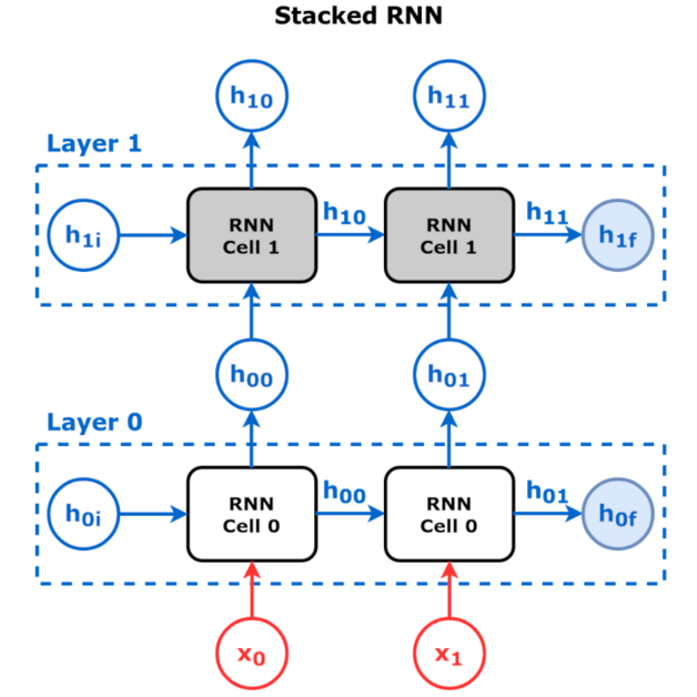
The main portion of the model lies in a Stacked RNN, label as RNN in the high level view. The RNN takes in two inputs, the input state and the previous hidden state, and returns an updated hidden state. This output is then fed into the next month of the model, as well as to the player state to make predictions with. A diagram of a stacked RNN in showed below.

Player Model and Output (Y)

The output of the RNN, the hidden stateh_x, is used to create the player state, and that state is used to create the outputs for the model. Once the model reaches the player state, it then diverges into predicting a number of different outputs. The player state then generates a number of pre-output states, which are then used to create a number of different outputs.

Once the model has reached the pre-output states, it is no longer a densely connected network with each node being influenced by each other node. For output M, outputs Y_M0 through Y_MN are generated only using pre-output states Z_M0 through Z_MN, and no influence from other pre-output blocks. This segregates each output into its own block, with this block translating the player state into a prediction that can be tested.

For the model outputs, they are done using classification using softmax to get the probability of each class. Doing classification for the predictions is done for two reasons. The first is that it allows for a probability distribution to be shown rather that just a number, so this model can differentiate between a player that is likely to be an MLB player but unlikely to be a star and a player who has a chance to be a star but is unlikely to make the show. The second is that the distribution of player outcomes is not normal: the range of Hitter WAR during control was -4.3 to 53.9. In training networks, using L2 loss (taking the error squared) generally gives better results than just the error, but in this case it would result in overvaluing players because a few superstars would generate a large model loss. Instead, WAR is put into a number of different buckets and the model generates a probability that the player ended up in each bucket.

The model currently generates 4 different outputs: WAR through control, peak seasonal WAR during control, the total PA/outs for a hitter/pitcher, and the highest level that a player achieved. Noteably, all of these are predicted during the same model run, and since all predictions converge at the player state to propogate their loss through the model, this results in errors in level prediction affecting the model for WAR prediction and vica versa. Somewhat surprisingly, predicting the player's level and the player's WAR generates a better WAR prediction than just predicting their WAR. The likely reason for this is that it allows for the model to better differentiate between players in the lower buckets; for the lowest—≤0 WAR—the player could have made the majors and had a few hundred PAs but not made it work, or they could have flamed out after hitting .150 in the DSL. While they both are in the same bucket, the MLB player was much closer to providing positive WAR than the DSL one, so this gives the model that insight between them.